How to Conduct Quantitative Research: Step by Step Guide

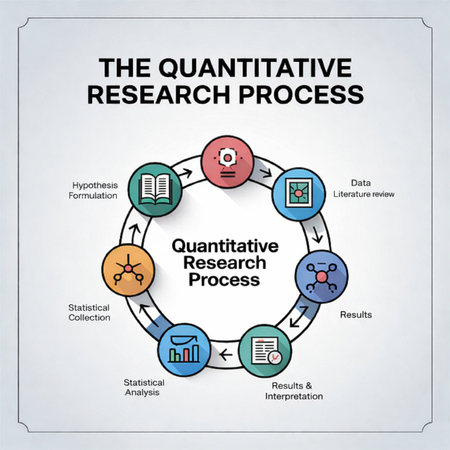
The Quantitative Research Process (Step by Step)

Quantitative research follows a structured, linear process. Here's your roadmap.

Step 1: Formulate Hypotheses

Unlike qualitative research, quantitative research typically tests hypotheses, not just research questions.

Research question format:

• "Is there a relationship between X and Y?"
• "Does X affect Y?" 
• "How much does X predict Y?"

Converting to hypotheses:

Research Question: "Is there a relationship between sleep and academic performance?"

Null Hypothesis (H?): There is no relationship between sleep hours and GPA.
Alternative Hypothesis (H?): There is a relationship between sleep hours and GPA.

Good hypotheses are:

• Testable with data
• Specific about variables 
• Directional when possible (positive/negative relationship) 
• Based on theory or prior research

Step 2: Select Your Research Design

Choose the design that matches your research question:

Experimental Design:

• Random assignment to conditions
• Manipulate independent variable 
• Measure dependent variable 
• Best for: Establishing causation

Quasi Experimental Design:

• No random assignment (existing groups)
• Manipulate or compare conditions 
• Best for: Natural settings where randomization isn't possible

Survey Research: 

• Collect data at one point in time
• No manipulation 
• Best for: Describing populations, examining relationships

Correlational Research: 

• Measure two or more variables
• No manipulation 
• Best for: Identifying relationships (not causation)

Longitudinal Research: 

• Measure same participants over time
• Best for: Tracking change and development

Step 3: Determine Sample Size

Sample size is critical in quantitative research. Too small = insufficient power; too large = wasted resources.

Power Analysis Method: Use G*Power (free software) to calculate needed sample size based on:

• Effect size: Small (d=0.2), Medium (d=0.5), Large (d=0.8)
•  Power: Typically 0.80 (80% chance of detecting real effect) 
•  Alpha: Typically 0.05 (5% chance of false positive) 
•  Statistical test: t-test, ANOVA, regression, etc.

General Guidelines:

For t-tests: 

• Small effect: approximately 310 per group
• Medium effect: approximately 64 per group
• Large effect: approximately 26 per group

For correlations: 

• Small effect: approximately 783 total
• Medium effect: approximately 85 total 
• Large effect: approximately 29 total

For regression (multiple predictors):

• Minimum: 10-15 participants per predictor variable
• Better: 20+ participants per predictor

For surveys: 

• Population < 100: Survey entire population
• Population 100-1,000: 50-80% sample 
• Population > 5,000: 400+ for 95% confidence level

Step 4: Design Data Collection Instruments

Your instrument (survey, test, observation protocol) must be valid and reliable.

For surveys:

• Use validated scales when available (e.g., PHQ 9 for depression, PSS for stress)
• Create new items only when necessary 
• Clear, unambiguous wording 
• Appropriate response scales
•  Pilot test with 20-30 people

For experiments:

• Clearly operationalize all variables
• Standardize procedures 
• Control extraneous variables 
• Plan manipulation checks

For structured observations:

• Clear behavioral definitions
• Train observers 
• Calculate inter rater reliability

Step 5: Select Sampling Method

Random Sampling Methods (best for generalization):

Simple Random Sampling:

• Every member has equal chance
• Use random number generator 
• Best for homogeneous populations

Stratified Random Sampling: 

• Divide population into strata (subgroups)
• Randomly sample from each stratum 
• Ensures representation of all groups

Cluster Sampling: 

• Randomly select clusters (schools, cities)
• Survey everyone in selected clusters 
• Cost effective for geographically dispersed populations

Systematic Sampling: 

• Select every nth person from list
• Easy to implement 
• Assumes list has no hidden patterns

Non Random Sampling Methods (convenient but less generalizable):

• Convenience Sampling: Whoever is available
• Snowball Sampling: Participants recruit participants
• Quota Sampling: Fill predetermined quotas for subgroups

Step 6: Collect Your Data

Best practices for data collection:

For online surveys: 

• Use professional platform (Qualtrics, SurveyMonkey, Google Forms)
• Test on multiple devices 
• Enable data validation (prevent invalid entries) 
• Send reminders (increases response rates) 
• Keep surveys under 15 minutes

For experiments:

• Follow protocol exactly
• Randomize presentation order when possible 
• Record all data immediately 
• Note any deviations from protocol 
• Blind data collection when possible

For in person data collection:

• Prepare materials in advance
• Have backup recording methods 
• Create comfortable environment
• Thank participants

Response Rate Strategies:

• Multiple contact attempts (3-5)
• Incentives ($5-25 gift cards) 
• Personalized invitations 
• Emphasize importance and ease 
• Follow up with non responders

Step 7: Clean and Prepare Data

Before analysis, clean your data:

Data entry checks:

• Import data into SPSS, R, or Excel
• Check for out of range values (e.g., age = 999) 
• Look for patterns of missing data 
• Verify reverse scored items

Handling missing data:

• Listwise deletion (delete entire case)
• Pairwise deletion (use available data) 
• Mean substitution (replace with variable mean) 
• Multiple imputation (advanced, creates multiple datasets)

Creating composite scores:

• Reverse score negatively worded items
• Calculate scale means or sums 
• Check internal consistency (Cronbach's alpha)

Data transformations: 

• Log transformation for skewed data
• Standardization (z scores) for comparing different scales 
• Dummy coding for categorical variables in regression

Step 8: Conduct Statistical Analysis

This is where quantitative data analysis happens. (Detailed in Section 3 below.)

Basic process:

1. Descriptive statistics (means, SDs, frequencies)
2. Check assumptions for your statistical test
3. Run inferential statistics 
4. Interpret results
5. Create tables and figures

Step 9: Interpret Results

Statistical significance (p-value): 

• p < .05: Result is statistically significant
• p ? .05: Result is not statistically significant 
• But: statistical is not equal to practical significance

Effect size: 

• Small, medium, or large effect
• More meaningful than p-value alone 
• Required in modern research

Confidence intervals: 

• Range where true value likely falls
• Provides more information than p-value 
• Report alongside point estimates

Step 10: Write Your Results

Quantitative results sections include:

• Sample characteristics (demographics table)
• Descriptive statistics (means, SDs) 
• Test results (test statistic, df, p-value, effect size) 
• Tables and figures 
• Text interpretation of findings

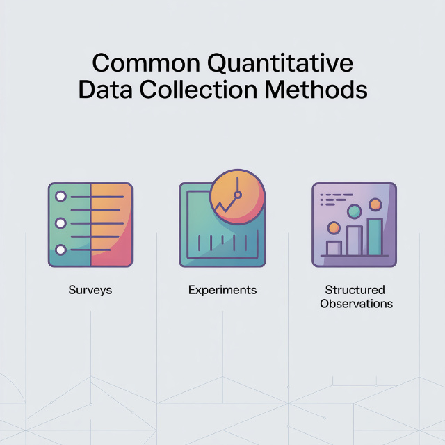
Detailed Data Collection Procedures

Let's dive deep into how to conduct quantitative research through specific data collection methods.

1. Designing Effective Surveys

Survey design is both art and science. Poor design = useless data.

Question Types:

1. Closed Ended Questions 

• Multiple choice: Select one option
• Checkboxes: Select all that apply 
• Likert scales: 1 (Strongly Disagree) to 5 (Strongly Agree) 
• Semantic differential: Rate between opposite adjectives 
• Ranking: Order items by preference

2. Demographic Questions

• Age, gender, education, income
• Place at end (less intrusive) 
• Provide "prefer not to answer" option

Question Writing Principles:

Likert Scale Best Practices:

Number of points:

• 5 point: Most common, sufficient for most purposes
• 7 point: More granularity, but harder for respondents
• 4 point or 6 point: Forced choice (no neutral option)

Labeling: 

• Label all points or just endpoints (research is mixed)
• Keep labels consistent throughout survey
• Avoid emotional language in labels

Response bias considerations: 

• Acquiescence bias: Tendency to agree (vary positive/negative items)
• Social desirability: Answering "correctly" (emphasize anonymity)
• Central tendency: Avoiding extremes (use forced choice or don't label middle)

Survey Structure:

1. Introduction: Purpose, time, confidentiality, contact info
2. Screening questions: Ensure eligibility
3. Easy questions first: Build confidence
4. Main questions: Organized by topic
5. Demographics: At end
6. Thank you: Appreciation and next steps
   
   

Pilot Testing:

• Test with 20-30 people from target population
• Check completion time
• Identify confusing questions
• Test skip logic and branching
• Calculate Cronbach's alpha for scales (? > .70 acceptable)

2. Designing Experiments

Experiments establish causation through controlled manipulation.

Key Components:

1. Independent Variable (IV):

• What you manipulate
• At least 2 levels (e.g., treatment vs. control)
• Clearly operationalized

2. Dependent Variable (DV):

• What you measure
• Valid and reliable measure
• Sensitive to change

3. Random Assignment:

• Participants randomly assigned to conditions
• Controls for confounding variables
• Essential for causation

4. Control:

• Control group receives no treatment or placebo
• All groups treated identically except IV 
• Standardized procedures

Experimental Designs:

Between Subjects Design:

• Different participants in each condition
• Need larger sample
• No practice effects
• Individual differences can confound

Within Subjects Design:

• Same participants in all conditions
• Smaller sample needed
• Control individual differences
• Risk of practice/fatigue effects

Mixed Design:

• Some IVs between subjects, some within subjects
• Combines advantages
• More complex analysis

Ensuring Internal Validity:

Control confounding variables:

• Standardize environment
• Use same equipment/materials
• Same researcher when possible
• Same time of day when possible

Random assignment:

• Use random number generator
• Stratify if needed (ensure groups balanced on key variables)
• Check that groups don't differ at baseline

Manipulation checks:

• Verify participants experienced intended manipulation
• Ask participants what they think study is about
• Check attention (catch questions)

Blinding:

• Single blind: Participants don't know condition
• Double blind: Neither participants nor experimenters know
• Reduces bias

Ethical Considerations:

Informed consent:

• Explain what they'll do
• Emphasize voluntary participation
• Right to withdraw anytime
• Debrief after if deception used

Minimizing harm:

• Risk should be minimal
• Benefits should outweigh risks
• Provide resources if sensitive topics

3. Structured Observations

Structured observation involves counting or rating pre defined behaviors.

Developing Observation Protocol:

1. Define behaviors clearly:

• Operational definitions
• Observable (not inferred)
• Mutually exclusive categories
• Exhaustive (covers all possibilities)

2. Choose recording method:

• Frequency count: How many times behavior occurs
• Duration: How long behavior lasts
• Interval recording: Did behavior occur during time interval?
• Rating scales: Rate intensity or quality

3. Train observers:

• Practice with videos
• Discuss borderline cases
• Continue until inter rater reliability is high

4. Calculate inter  rater reliability:

• Cohen's kappa (? > .70 acceptable) 
• Percent agreement
• Intraclass correlation

5. Minimize reactivity:

• Allow adjustment period (people get used to observer)
• Unobtrusive positioning
• Explain observations as "normal procedure"

4. Secondary Data Analysis

Secondary data analysis uses existing datasets.

Sources:

• Government databases (Census, NCES, BLS)
• Previous research datasets (ICPSR, Harvard Dataverse) 
• Institutional records (student data, health records) 
• Social media data (Twitter API, Reddit)

Advantages:

• Cost effective (often free)
• Large samples 
• High quality data (professionally collected) 
• Can answer questions you couldn't collect yourself

Challenges:

• Limited by original collection methods
• May not have exact variables you want 
• Need to understand original context 
• Requires data use agreements

Best Practices:

• Thoroughly understand data collection methods
• Check data quality and missingness 
• Cite original source properly 
• Consider limitations in interpretation

Statistical Analysis Techniques

This is where quantitative data analysis happens. Here are the essential techniques.

1. Descriptive Statistics

Descriptive statistics summarize and describe your data.

Measures of Central Tendency:

Measures of Variability:

2. Inferential Statistics: Comparing Groups

Inferential statistics test hypotheses and make inferences about populations.

Independent Samples t-test

Purpose: Compare means of two independent groups

Example: Do males and females differ in stress levels?

Assumptions: 

• Independent observations
• Normally distributed within groups
• Homogeneity of variance

SPSS: Analyze, Compare Means, Independent Samples T-Test

Paired Samples t-test

Purpose: Compare means of same group at two time points

Example: Did stress decrease from pre test to post test?

Assumptions:

• Paired observations
• Normally distributed difference scores

SPSS: Analyze, Compare Means, Paired Samples T-Test

One Way ANOVA (Analysis of Variance)

Purpose: Compare means of three or more groups

Example: Do freshmen, sophomores, juniors, and seniors differ in stress?

Post hoc tests:

• Tukey HSD: When equal sample sizes
• Games Howell: When unequal variances
• Bonferroni: Conservative, controls Type I error

SPSS: Analyze, Compare Means, One Way ANOVA

Two Way ANOVA

Purpose: Examine effects of two independent variables and their interaction

Example: Do gender and year in school affect stress? Is there an interaction?

SPSS: Analyze, General Linear Model, Univariate

Chi Square Test

Purpose: Test associations between categorical variables

Example: Is there a relationship between gender and major choice?

Assumptions:

• Independent observations
• Expected frequencies ? 5 in each cell

SPSS: Analyze, Descriptive Statistics, Crosstabs, Statistics, Chi square

3. Inferential Statistics: Examining Relationships

Pearson Correlation

Purpose: Measure strength and direction of linear relationship between two continuous variables

Correlation coefficient (r):

• Range: ?1 to +1
• Interpretation:
  • 0.1–0.3: Small
  • 0.3–0.5: Medium
  • 0.5–1.0: Large

Assumptions:

• Linear relationship
• Normally distributed
• No significant outliers

SPSS: Analyze, Correlate, Bivariate

Spearman Correlation

Purpose: Measure relationship for ordinal data or non normal distributions

Use when: Data is ranked or severely skewed

Simple Linear Regression

Purpose: Predict one variable from another

Provides:

• How much variance explained (R²)
• Prediction equation
• Significance of predictor

SPSS: Analyze, Regression, Linear

Multiple Regression

Purpose: Predict one variable from multiple predictors simultaneously

Advantages:

• Control for confounding variables
• Determine relative importance of predictors
• More realistic models

Types:

• Standard (simultaneous): All predictors entered at once
• Hierarchical: Enter predictors in blocks
• Stepwise: Software selects predictors (use cautiously)

SPSS: Analyze, Regression, Linear

4. Checking Assumptions

Before running statistical tests, check assumptions:

Normality:

• Visual: Histogram, Q Q plot
• Statistical: Shapiro Wilk test (p > .05 = normal) 
• If violated: Transform data or use non parametric tests

Homogeneity of variance:

• Levene's test (p > .05 = equal variances)
• If violated: Use Welch's correction or non parametric tests

Independence: 

• Design based (e.g., each participant measured once)
• If violated: Use repeated measures or multilevel models

Linearity (for correlation/regression): 

• Scatterplot should show linear pattern
• If violated: Transform variables or use non linear models

No multicollinearity (regression):

• VIF < 10 (preferably < 5)
• If violated: Remove correlated predictors

Non Parametric Alternatives:

When assumptions violated:

• Mann Whitney U (instead of t-test)
• Wilcoxon signed rank (instead of paired t-test) 
• Kruskal Wallis (instead of ANOVA) 
• Spearman correlation (instead of Pearson)

Software and Tools

Statistical software is essential for quantitative research. Here's what you need to know.

1. SPSS (Most User Friendly)

Best for: Students, beginners, standard analyses

Pros: 

• Point and click interface (no coding)
• Widely used in social sciences
• Excellent documentation and tutorials
• Produces APA formatted tables
• Handles data management well

Cons: 

• Expensive ($100/month or $3,000+ perpetual license)
• Limited advanced modeling
• Less flexible than R

Common analyses: 

• Descriptive statistics
• t-tests, ANOVA, chi square
• Correlation, regression
• Factor analysis
• Reliability analysis

Learning curve: Low (1-2 weeks for basics)

Where to learn: LinkedIn Learning, YouTube, university workshops

2. R (Most Powerful, Free)

Best for: Advanced analyses, data visualization, researchers with programming skills

Pros: 

• Completely free and open source
• Unlimited statistical capabilities
• Beautiful visualizations (ggplot2)
• Reproducible research (R Markdown)
• Largest statistical community

Cons: 

• Steep learning curve (requires coding)
• Can be frustrating for beginners
• Requires package management

Common analyses: 

Everything SPSS does, plus:

• Advanced modeling (SEM, multilevel, machine learning)
• Publication quality graphics
• Automated reporting

Learning curve: Moderate High (2-3 months for proficiency)

Where to learn: DataCamp, Coursera, R for Data Science book

Essential packages: 

• tidyverse (data manipulation)
• ggplot2 (visualization)
• psych (psychological research)
• lme4 (multilevel models)

3. SAS (Industry Standard)

Best for: Large datasets, complex analyses, industry research

Pros: 

• Handles massive datasets
• Excellent for complex models
• Industry standard (healthcare, finance)
• Superior data management
• Strong technical support

Cons: 

• Very expensive
• Steep learning curve
• Less intuitive interface
• Smaller academic user base

Learning curve: High (3-6 months)

4. Stata (Popular in Economics/Social Sciences)

Best for: Panel data, econometrics, social science research

Pros: 

• Balance between SPSS and R
• Excellent for longitudinal data
• Good documentation
• Command based but learnable
• One time purchase

Cons: 

• Expensive ($1,500–5,000)
• Steeper than SPSS
• Smaller user community than R/SPSS

Learning curve: Moderate (1-2 months)

5. Excel (Basic Statistics Only)

Best for: Simple descriptive statistics, data organization

Pros: 

• Everyone has it
• Familiar interface
• Good for data entry and cleaning
• Basic statistics available

Cons: 

• Limited statistical capabilities
• Not designed for research
• Easy to make errors
• Poor for large datasets

Use for: 

• Data entry
• Basic descriptives (mean, SD)
• Simple correlations
• Pivot tables

Don't use for: Anything requiring inferential statistics

6. Choosing Software

Decision tree:

Complete Research Examples

Let's see quantitative research examples with strong methodology sections.

Example 1: Survey Research

Example 2: Experimental Research

Example 3: Quasi Experimental Research

Common Challenges (And Solutions)

Every quantitative researcher faces these challenges. Here's how to solve them.

Challenge 1: Determining Sample Size

The Problem: "How many participants do I need?"

Solutions: 

• Always conduct power analysis using G*Power
• Report power analysis in methodology
• Consider practical constraints (time, money, access)
• Err on side of larger sample when possible
• If sample ends up smaller, acknowledge as limitation

Quick reference: 

• Small effects require 300+ participants
• Medium effects require 60–85 participants
• Large effects require 25–30 participants

Challenge 2: Low Response Rates

The Problem: 10-20% response rate undermines generalizability.

Solutions: 

• Multiple contacts: Initial invite + 3–4 reminders
• Incentives: Even small ($5) increases response
• Personalization: Use names, explain why they specifically were selected
• Timing: Send mid week, mid morning
• Emphasis: Stress importance and how long it takes
• Mobil friendly: Most people check email on phones

Target: 30-40% response rate minimum

Challenge 3: Choosing the Right Statistical Test

The Problem: "Which test do I use?"

Solutions:

Decision tree:

Challenge 4: Dealing with Missing Data

The Problem: Participants skip questions or drop out.

Solutions:

Prevention: 

• Make all survey questions required (except sensitive items)
• Keep surveys short
• Provide “prefer not to answer” option

After the fact: 

• < 5% missing: Listwise deletion acceptable
• 5–20% missing: Check if missing at random, consider imputation
• 20% missing: Results may be biased, report as limitation

Analysis options: 

• Listwise deletion (delete entire case)
• Pairwise deletion (use available data)
• Mean substitution (replace with variable mean – not recommended)
• Multiple imputation (advanced, best practice)

Challenge 5: Non Normal Data

The Problem: Data is severely skewed, violates normality assumption.

Solutions:

Check severity:

• Shapiro–Wilk test (p < .05 = non normal)
• Visual inspection (histogram, Q–Q plot)
• Skewness and kurtosis values

Options:

1. Transform data: Log, square root, or reciprocal transformation
2. Use non parametric tests: Mann–Whitney U, Kruskal–Wallis
3. Increase sample size: Central limit theorem (n > 30 helps)
4. Accept violation: t-tests and ANOVA fairly robust to mild violations

Challenge 6: Interpreting Non Significant Results

The Problem: p > .05, but you expected significance.

Possible reasons: 

• Insufficient power (sample too small)
• No real effect exists (null is true)
• Poor measurement (unreliable instruments)
• Too much variability (large standard deviations)

What to do: 

• Check power post hoc
• Examine effect size (maybe effect exists but is small)
• Don’t p hack (run multiple tests until something is significant)
• Report honestly and discuss implications

Challenge 7: Meeting SPSS/Software Requirements

The Problem: Never used statistical software before.

Solutions:

For SPSS: 

• Start with YouTube tutorials (“SPSS for beginners”)
• Use built in tutorials (Help, Tutorial)
• Practice with sample datasets
• Ask for help early (advisor, stats consultant, classmates)

For R: 

• Start with RStudio
• Follow DataCamp or Coursera courses
• Practice with tidyverse packages
• Join R community (Stack Overflow, R for Data Science)

Bottom Line

Conducting quantitative research requires careful planning, rigorous execution, and appropriate statistical analysis. The key is matching your research design to your question, collecting high quality data, and analyzing it with the right statistical tools.

Remember:

• Power analysis determines your sample size
• Valid, reliable instruments are essential
• Random sampling enables generalization
  
• Check assumptions before running tests
  
• Effect sizes matter more than p-values
  
• Statistical significance is not equal to practical importance
  
• Software helps, but understanding statistics is crucial

Whether you execute quantitative research yourself or get expert support, the goal is producing valid, reliable findings that advance knowledge.

For broader methodology context, see our research methodology guide.

Good luck with your quantitative research!